Differential Geometry

Textbook: Visual Differential Geometry and Forms: A Mathematical Drama in Five Acts by Tristan Needham

1-Forms

1. Basic definitions: A linear, real-valued function of a single vector input, $\omega :V\to \mathbb{R}$. The addition and (scalar) multiplication of 1-forms can be naturally defined that the set of all 1-forms constitute a vector space, the dual to $V$. Then $v(\omega ):=\omega (v)$(contraction, see below).
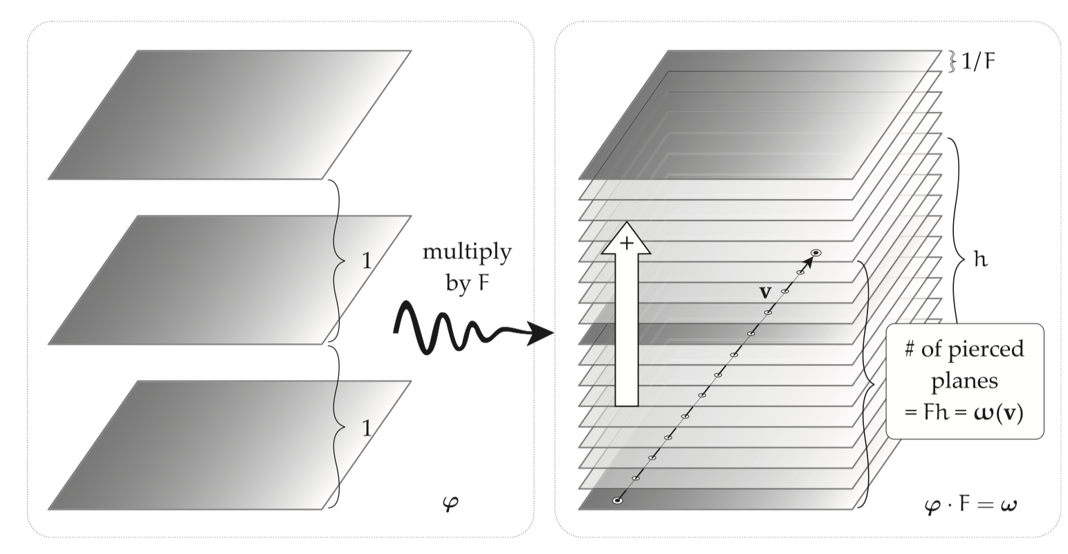
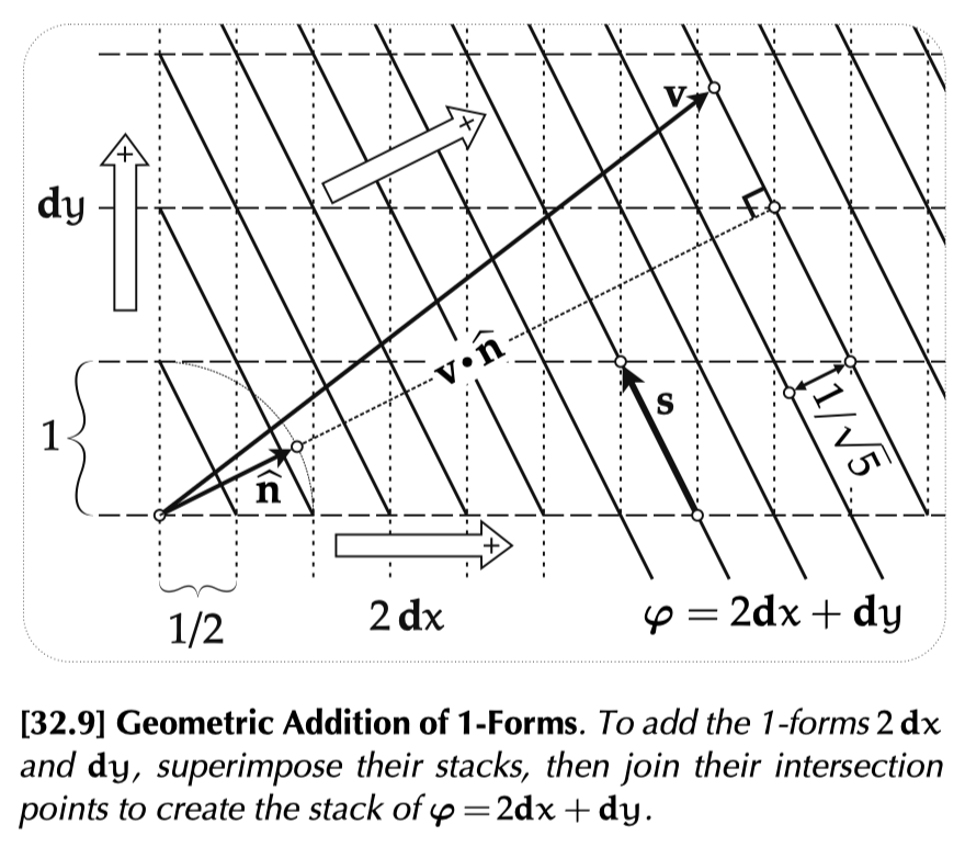
   1. Visualisation: A ground plane defined by $\omega (v)=0$ and a stack of parallel planes defined by $\omega (v)=h$. By adjusting the spacing of planes (to be $\frac{1}{\omega (1)}$) we can make $\omega (v)=\#\text{planes pierced by }v$.
   2. Gradient 1-form: Recall that in a topographic map, the steepness is inversely proportional to the (smallest) distance between neighbouring contours, $steepness={\sup }_{\delta s}\frac{\delta h}{\delta s}\sim {\sup }_{ds}\frac{dh}{ds}={\sup }_{|v|=1}\nabla f\cdot v=|\nabla f|$(reaches equal iff $v\parallel \nabla f$). Let $\zeta$ to be a (1-form) field that ${\zeta }_p$ is an 1-form defined by ${\zeta }_p(v)=(\#\text{projected contour pierced by }v)\cdot \delta h$ in the immediate vicinity of $p$.
2. Basis 1-forms: Consider a basis $\{e_j\}$ for $T_p$ and the dual basis $\{{\omega }^i\}$ for $T_p^{\ast }$, in which ${\omega }^i(v)=v^i$(An equivalent definition being ${\omega }^i(e_j)={\delta }_j^i$). Actually any 1-form $\phi$ satisfies $\phi =\sum \phi (e_j){\omega }^j$.
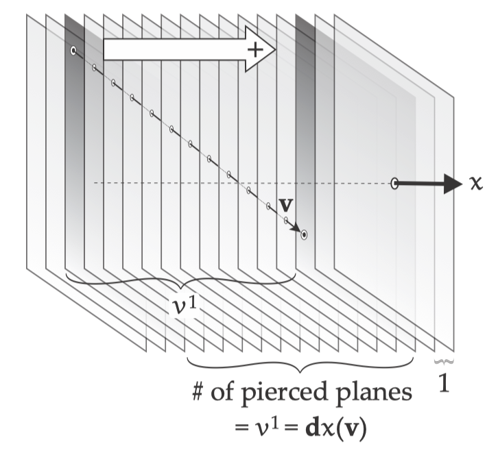
3. The gradient as a 1-form: $df(v):={\nabla }_{v}f$($d$=exterior derivative).
   1. $d{x}^j(v)=\left(\sum v^i\frac{\partial }{\partial x^i}\right)x^j=v^j$ where $x^j$ is an operator to extract the $j$-th coordinate of $v\in {\mathbb{R}}^n$. Note that formally $d{x}^j$ has a same effect but act on a direction $v\in T_{p}M$ and means the change rate of $x^j$ on direction $v$. We call $\{d{x}^j\}=\{{\omega }^j\}$ the Cartesian basis of 1-forms dual to $\{e_j\}$.
   2. Substitue $\phi =df$ in, $df=\sum (df(e_i))d{x}^j=\sum \frac{\partial f}{\partial x^j}d{x}^j$.
   3. Geometric meaning: Consider a manifold characterised by $\{(x,f(x))\in {\mathbb{R}}^n\times \mathbb{R}\}$. Apply the definition of ${\zeta }_p(v)$ then $\zeta =df$.
4. Geometric intuition of 1-forms: Multiply by $k$ <-> compress the stack by $k$; Simple calculations shows that the addition($2dx+dy$ for example) of 1-forms is itself a 1-form corresponding to a new stack constructed like the figure shows.

Tensors

1. Definitions: A tensor $H({\phi }_1,\cdots ,{\phi }_f\Vert v_1,\cdots ,v_v)$ of valence $\left\{\begin{array}{c}f\\ v\end{array}\right\}$ at $p$ is a multilinear, real-valued function of $f$ 1-forms and $v$ vectors. Its value at $p$ only depends on the value of 1-forms and vectors at $p$. $H:(T_p^{\ast }M{)}^f\times (T_{p}M{)}^v\to {\mathbb{R}}^n$.
   1. Operation: For tensors with a same valence, addition can be defined naturally; The tensor product is defined as $(\phi \otimes \psi )(v,w):=\phi (v)\psi (w)$ for $\left\{\begin{array}{c}0\\ 1\end{array}\right\}$ tensors(1-forms). Then simply $(J\otimes T)(\cdots )=J(\cdots )T(\cdots )$ for tensors of general valences.
2. Components: $T_{ij}:=T(e_i,e_j)$, then $T(v,w)=\sum T_{ij}{v}^i{w}^j=\sum T_{ij}(d{x}^i\otimes d{x}^j)(v,w)$, or $T=\sum T_{ij}(d{x}^i\otimes d{x}^j)$. Directly we see that $\{d{x}^i\otimes d{x}^j\}$ forms a basis for tensors of valance $\left\{\begin{array}{c}0\\ 2\end{array}\right\}$. Similarly consider $(v\otimes w)(\phi ,\psi )=\sum v^i{w}^j(e_i\otimes e_j)(\phi ,\psi )$ and $\{e_i\otimes e_j\}$ as a basis for $\left\{\begin{array}{c}2\\ 0\end{array}\right\}$s. Generally we may decompose $\left\{\begin{array}{c}f\\ v\end{array}\right\}$s using the basis $\{(e_{i_1}\otimes \cdots \otimes e_{i_f})\otimes (d{x}^{j_1}\otimes \cdots \otimes d{x}^{j_v})\}$.
3. Changing val:
   1. Contraction: $\phi (v)=\left(\sum {\phi }_{i}d{x}^j\right)\left(\sum v^j{e}_j\right)=\sum ({\phi }_i{v}^j)(d{x}^i{e}_j)=\sum {\phi }_i{v}^j$, independent of the specific components of $\phi ,v$(trace of a matrix). Now suppose a general case of $A\otimes B$. When summing over an upper index(contravariant) of $A$ and a lower index(covariant) of $B$(i.e. $\sum A^{ij}{B}_{jk}$), we get another tensor (1) whose valance has each index reduced by 1 compared to that of $A\otimes B$, (2) which is independent of the choice of basis.
   2. Metric tensor: Consider a metric tensor $g$ of valence $\left\{\begin{array}{c}0\\ 2\end{array}\right\}$ and a map from vector $n$ to 1-form $\nu$ that $\nu (w):=g(w,n)$. Calculation shows that $\nu =\sum n_{i}d{x}^i$ where $n_i=\sum g_{ij}{n}^j$. Let, e.g. $R(u,v,w,n)=R(\nu \Vert u,v,w)$ then $R_{ijkl}={\sum }_m{R}_{ijk}^m{g}_{ml}$. The process in called index lowering. Correspondingly we can take $\tilde{g}$ of valence $\left\{\begin{array}{c}2\\ 0\end{array}\right\}$ to define $n(\phi ):=\tilde{g}(\phi ,\nu )$ to do index raising.

2-Forms

1. Basic definitions: A 2-form $\Psi$ is an antisymmetric tensor of valence $\left\{\begin{array}{c}0\\ 2\end{array}\right\}$, that is $\Psi (v,u)=-\Psi (u,v)$. A p-form is a completely antisymmetric tensor of valence $\left\{\begin{array}{c}0\\ p\end{array}\right\}$, meaning that swapping any two of the inputs reverses the sign.
   1. $\mathcal{A}(u,v):=\text{oriented area of the parallelogram with edges }u,v$. Obviously $\mathcal{A}$ is a 2-form.
   2. Wedge product: We can split $\phi \otimes \psi$ into the sum of a symmetric tensor and an antisymmetric tensor and define the latter to be the wedge product, i.e. $\phi \wedge \psi :=\phi \otimes \psi -\psi \otimes \phi$. Besides the inputs, we have the antisymmetry of the wedge product itself $\phi \wedge \psi =-\psi \wedge \phi$.
   3. $\mathcal{A}=dx\wedge dy$. In a general case, $(\phi \wedge \psi )(v_1,v_2)=\mathcal{A}(F(v_1),F(v_2))$.
2. Basis: $\{d{x}^i\wedge d{x}^j:i<j\}$ constitutes a basis for the 2-forms. $\Psi ={\Psi }_{12}(dx\wedge dy)$ for ${\mathbb{R}}^2$ and $\Psi ={\Psi }_{23}(dy\wedge dz)+{\Psi }_{31}(dz\wedge dx)+{\Psi }_{12}(dx\wedge dy)$ for ${\mathbb{R}}^3$.
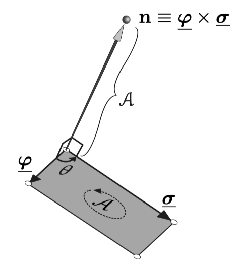
3. Flux: Let $\underline{\Psi }=\left(\begin{array}{c}{\Psi }^1\\ {\Psi }^2\\ {\Psi }^3\end{array}\right)=\left(\begin{array}{c}{\Psi }_{23}\\ {\Psi }_{31}\\ {\Psi }_{12}\end{array}\right)$. Now imagine a uniform flow of fluid with velocity $\underline{\Psi }$ and define $\Phi (v_1,v_2)=\text{Amount of fluid crossing P per unit time}=\text{flux of }\underline{\Psi }\text{ through P}$. The flux is positive iff the direction of P and $\underline{\Psi }$ is on the same side. By simple calculation we find that $\Phi =\Psi$.
4. Vector and wedge products: Let $\underline{\phi }=\left(\begin{array}{c}{\phi }_1\\ {\phi }_2\\ {\phi }_3\end{array}\right)$ where $\phi ={\phi }_{1}d{x}^1+{\phi }_{2}d{x}^2+{\phi }_{3}d{x}^3$. Then $\underline{\Psi }=\underline{\phi }\times \underline{\sigma }$ where $\Psi =\phi \wedge \sigma$, or $\underline{\Psi }=\Psi$. This holds in and only in ${\mathbb{R}}^3$ where $\frac{1}{2}n(n-1)=n$.
   1. The volume of a parallelepiped with edges $u,v,\underline{\Omega }$: Volume=flux=$\Omega (u,v)=\left(\begin{array}{c}{\Omega }^1\\ {\Omega }^2\\ {\Omega }^3\end{array}\right)\cdot \left(\begin{array}{c}{u}^2{v}^3-u^3{v}^2\\ u^3{v}^1-u^1{v}^3\\ u^1{v}^2-u^2{v}^1\end{array}\right)=\det \left(\begin{array}{ccc}\underline{\Omega }& u& v\end{array}\right)$.
5. The Faraday and Maxwell electromagnetic 2-forms: Consider electric field $\underline{E}=\left(\begin{array}{c}{E}_x\\ E_y\\ E_z\end{array}\right)$ and magnetic field $\underline{B}=\left(\begin{array}{c}{B}_x\\ B_y\\ B_z\end{array}\right)$. The corresponding 2-forms and 1-forms: E = E_{x}(dy \wedge dz) + E_{y}(dz \wedge dx) + E_{z}(dx \wedge dy),\quad \varepsilon=E_{x}dx+E_{y}dy+E_{z}dz, $$$$B = B_{x}(dy \wedge dz) + B_{y}(dz \wedge dx) + B_{z}(dx \wedge dy),\quad \beta=B_{x}dx+B_{y}dy+B_{z}dz. Now define Faraday 2-form $F=\epsilon \wedge dt+B$, Maxwell 2-form $\star F=\beta \wedge dt-E$, both in $4$ dimensions. Actually here $\star$ means Hodge dual.

3-Forms

1. The wedge product of a 2-form and 1-form: $(\Psi \wedge \sigma )(v_1,v_2,v_3):=\Psi (v_1,v_2)\sigma (v_3),\Psi (v_3,v_1)\sigma (v_2)+\Psi (v_2,v_3)\sigma (v_1)$. Note that $\Psi \wedge \sigma =\sigma \wedge \Psi$. Generally if $\Psi$ is a $p$-form and $\Omega$ is a $q$-form, then $\Psi \wedge \Omega =(-1{)}^{pq}\Omega \wedge \Psi$.
2. The volume 3-form: Easy to verify $\mathcal{V}(u,v,\underline{\Omega })=\Omega (u,v)$ where $\mathcal{V}=d{x}^1\wedge d{x}^2\wedge d{x}^3$.
3. The wedge product of three(and more) 1-forms is associative: We can write without ambiguity $\underset{1}{\sigma }\wedge \underset{2}{\sigma }\wedge \underset{3}{\sigma }$. Geometrically thinking, we can also define $F:v\mapsto \left(\begin{array}{c}\underset{1}{\sigma }(v)\\ \underset{2}{\sigma }(v)\\ \underset{3}{\sigma }(v)\end{array}\right)$ and $\underset{1}{\sigma }\wedge \underset{2}{\sigma }\wedge \underset{3}{\sigma }:(v_1,v_2,v_3)\mapsto \det \left(\begin{array}{ccc}F(v_1)& F(v_2)& F(v_3)\end{array}\right)$. This definition can be generalised to the wedge product of $p$ 1-forms.
   1. Abstract definition of wedge product: (1) Bilinearity (2) associativity and (3) graded antisymmetry are enough to determine the operation.
   2. Explicit formula: $(\phi \wedge \psi )(v_1,\cdots ,v_{p+q})=\frac{1}{p!q!}{\sum }_{\sigma \in S_{p+q}}\mathrm{sgn}(\sigma )\phi (v_{\sigma (1)},\cdots ,v_{\sigma (p)})\psi (v_{\sigma (p+1)},\cdots ,v_{\sigma (p+q)})$.
4. Basis: $\{d{x}^{i_1}\wedge \cdots \wedge d{x}^{i_p}:i_1<\cdots <i_p\}$ forms a basis for $p$-forms.

Differentiation

1. The exterior derivative: Concentrating on one point $p\in M$, a 0-form is a scalar. Then for different $p$s these scalars constitutes a function(scalar field) $f$. The exterior derivative $d$ increases the degree of the form by one to allow for the input of an additional vector(direction). Similarly we can take an 1-form field $\phi$ and vector field $u,v$ to define $d\phi (u,v)={\nabla }_u\phi (v)-{\nabla }_v\phi (u)-\phi ([u,v])$, where the commutator $[u,v]:={\nabla }_{u}v-{\nabla }_{v}u$(we subtract this term to ensure the independence of the variations of the vector fields).
   1. Simplification of $d\phi$: Choose the vector fields to be constant and basis to be $\{d{x}^k\}$. Then $d\phi =\sum {\partial }_i{\phi }_j(d{x}^i\wedge d{x}^j)=\sum d{\phi }_j\wedge d{x}^j$.
   2. $p$-forms: $d\Phi =\sum d{\Phi }_{i_1,\cdots ,i_p}\wedge (d{x}^{i_1}\wedge \cdots d{x}^{i_p})=\sum d{x}^j\wedge {\partial }_j\Phi$.
2. The Leibniz rule: $d(\Phi \wedge \Psi )=(d\Phi )\wedge \Psi +(-1{)}^{\mathrm{deg}\Phi }\Phi \wedge (d\Psi )$.
   1. Another way to define $d$: A linear operator satisfying (1) the Leibniz rule (2) the equation of total derivative for functions(0-forms).
3. Closed and extra forms:
   1. $d^2=0$: We start from $d^2\phi =\sum d({\partial }_i{\phi }_j)\wedge d{x}^i\wedge d{x}^j=\sum ({\partial }_k{\partial }_i{\phi }_{j}d{x}^k\wedge d{x}^i)\wedge d{x}^j=0$ for a 2-form $\phi$. By induction we can verify $d^2\Phi$ holds for $\Phi$ of every degrees of form.
   2. Definition: ${\rm Y}$ is closed <-> $d{\rm Y}=0$, ${\rm Y}$ is exact <-> $\exists \text{potential }\Psi ,{\rm Y}=d\Psi$.
      1. Poincare Lemma: If a closed ${\rm Y}$ is defined on a simply connected region, then it’s also exact.
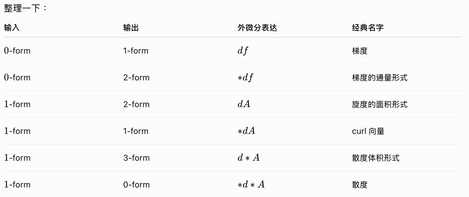
4. Vector calculus via forms: $\underline{d\phi }=\left(\begin{array}{c}{\partial }_2{\phi }_3-{\partial }_3{\phi }_2\\ {\partial }_3{\phi }_1-{\partial }_1{\phi }_3\\ {\partial }_1{\phi }_2-{\partial }_2{\phi }_1\end{array}\right)=\nabla \times \underline{\phi }:=\mathrm{curl}\underline{\phi }$. $d\Psi =\left(\begin{array}{c}{\partial }_1\\ {\partial }_2\\ {\partial }_3\end{array}\right)\cdot \left(\begin{array}{c}{\Psi }^1\\ {\Psi }^2\\ {\Psi }^3\end{array}\right)d{x}^1\wedge d{x}^2\wedge d{x}^3=(\nabla \cdot \underline{\Psi })\cdot \mathcal{V}=:(\mathrm{div}\underline{\Psi })\mathcal{V}$.
   1. Applying $d^2=0$ to $\phi =df,\Psi =d\phi$ we have $\nabla \times \nabla f=0,\nabla \cdot (\nabla \times \underline{\phi })=0$.
   2. Calculation including $\nabla \cdot$ and $\nabla \times$ can be translated to the language of forms. (usually with the lemma that $\phi \wedge \Psi =(\underline{\phi }\cdot \underline{\Psi })\mathcal{V}$)
5. Maxwell’s equations: ($d_S$ denotes the spatial part of the spacetime $d$, i.e. $df=d_{S}f+{\partial }_{t}fdt$)
   1. Source-free equations: $\nabla \cdot \underline{B}=0,\nabla \times \underline{E}+{\partial }_t\underline{B}=0$. Consider $dF=d(\epsilon \wedge dt)+dB=((\text{flux 2-form of }\nabla \times \underline{E})\wedge dt)+((\nabla \cdot \underline{B})\mathcal{V}+dt\wedge {\partial }_{t}B)=(\nabla \cdot \underline{B})\mathcal{V}+(\text{flux 2-form of }\nabla \times \underline{E}+{\partial }_t\underline{B})\wedge dt$. Then $F$ is closed. Applying Poincare lemma we know locally there exists a 1-form potential $A$ s.t. $F=dA$.
   2. Source equations(in Gaussian units): $\nabla \cdot \underline{E}=4\pi \rho ,\nabla \times \underline{B}-{\partial }_t\underline{E}=4\pi \underline{j}$. Similarly we have $d\star F=4\pi \star J$, where $J=-\rho dt+j$ and $\star J=-\rho \mathcal{V}+(\text{flux 2-form of }\underline{j})\wedge dt$.

Integration

1. The line integral of a 1-form: ${\int }_K\phi :={\mathcal{C}}_K(\underline{\phi })={\int }_K\underline{\phi }\cdot dr=\lim \sum \underline{\phi }\cdot \delta r=\lim \sum \phi (\delta r)$.
   1. Path-independence <-> vanishing loop integrals.
   2. Exact form: Let $\phi =df$. Substitute $\phi (\delta r)=df(\delta r)\sim \delta f$ into the definition, we have ${\int }_{K}df=f(b)-f(a)$.
2. The exterior derivative as an integral:
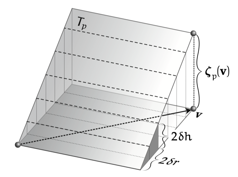
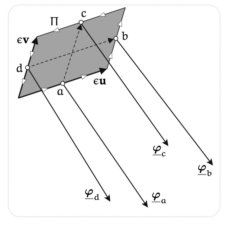
   1. $d(\text{1-form})$: Circulation $\Omega (\epsilon u,\epsilon v):={\oint }_{\Pi (\epsilon u,\epsilon v)}\phi$. We can evaluate $\Omega$ using the midpoints: $\Omega (\epsilon u,\epsilon v)\sim {\phi }_a(\epsilon u)+{\phi }_b(\epsilon v)+{\phi }_c(-\epsilon u)+{\phi }_d(-\epsilon v)\sim {\nabla }_{\epsilon u}\phi (\epsilon v)-{\nabla }_{\epsilon v}\phi (\epsilon u)$. Note here $u,v$ are vector fields and need not to be constant. The parallelogram is closed yields that ${\Phi }_{\epsilon }^v\circ {\Phi }_{\epsilon }^u-{\Phi }_{\epsilon }^u\circ {\Phi }_{\epsilon }^v=0$. Taylor expand shows that ${\Phi }_{\epsilon }^u(x)=x+\epsilon u(x)+\frac{{\epsilon }^2}{2}(u\cdot \nabla )u+O({\epsilon }^3)$. Necessarily the coefficient of ${\epsilon }^2$ vanishes, i.e $(u\cdot \nabla )v-(v\cdot \nabla )u=0$ or $[\epsilon u,\epsilon v]=0$(Frobenius theorem ensures that this is also a sufficient condition). Thus $\Omega (\epsilon u,\epsilon v)\sim d\phi (\epsilon u,\epsilon v)=(\nabla \times \underline{\phi })\cdot \hat{n}\mathcal{A}(\epsilon u,\epsilon v)$, or the circulation ultimately equals to the flux.
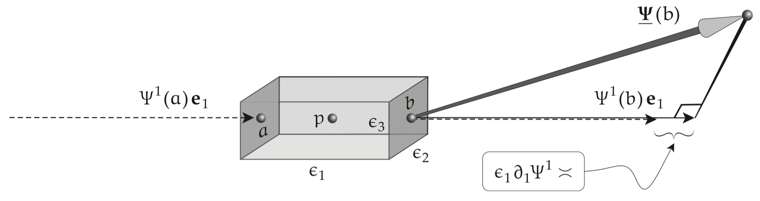
   2. $d(\text{2-form})$: Outward flux $\Omega (\epsilon u,\epsilon v,\epsilon w):={\iint }_{\Pi (\epsilon u,\epsilon v,\epsilon w)}\Psi \sim d\Psi (\epsilon u,\epsilon v,\epsilon w)=(\nabla \cdot \underline{\Psi })\mathcal{V}(\epsilon u,\epsilon v,\epsilon w)$.
3. Fundamental theorem of exterior calculus(generalised Stokes’s theorem): ${\int }_{R}d\Phi ={\int }_{\partial R}\Phi$.
   1. Area: ${\oint }_{\partial R}xdy=\sum {\oint }_{\partial (\delta R)}xdy$, here $\delta R$ is a rectangle stripped from $R$ parallel to $x$-axis. Obviously ${\oint }_{\partial (\delta R)}xdy=\delta x\delta y=\mathcal{A}(\delta R)$ then ${\oint }_{\partial R}xdy=\mathcal{A}(R)$. Applying FTEC directly we have ${\oint }_{\partial R}xdy={\iint }_{R}d(xdy)={\iint }_{R}dx\wedge dy=\mathcal{A}(R)$.
   2. ${\partial }^2=0$: Applying FTEC twice yields $0={\int }_R{d}^2\Phi ={\int }_{\partial R}d\Phi ={\int }_{{\partial }^{2}R}\Phi$ for every $\Phi ,R$ , then ${\partial }^2=0$. Conversely $d^2=0$ if we know ${\partial }^2=0$.
   3. 0-form(Newton-Leibniz): ${\int }_{K}df=f(b)-f(a)$.
   4. 1-form:
      1. Green’s theorem: $d\phi =d{\phi }_1\wedge d{x}^1+d{\phi }_2\wedge d{x}^2={\partial }_2{\phi }_{1}d{x}^2\wedge d{x}^1+{\partial }_1{\phi }_{2}d{x}^1\wedge d{x}^2=({\partial }_1{\phi }_2-{\partial }_2{\phi }_1)d{x}^1\wedge d{x}^2$. Then ${\oint }_{\partial R}{\phi }_{1}d{x}^1+{\phi }_{2}d{x}^2={\oint }_{\partial R}\phi ={\iint }_{R}d\phi ={\iint }_R({\partial }_1{\phi }_2-{\partial }_2{\phi }_1)d{x}^1\wedge d{x}^2$.
      2. Stokes’s theorem: ${\oint }_{\partial S}\underline{\phi }\cdot dr={\oint }_{\partial S}\phi ={\iint }_{S}d\phi ={\iint }_S(\nabla \times \underline{\phi })\cdot \hat{n}d\mathcal{A}$.
   5. 2-form(Gauss’s/divergence theorem): ${\iiint }_V(\nabla \cdot \underline{\Psi })d\mathcal{V}={\iiint }_{V}d\Psi ={\oint }_{\partial V}\Psi ={\oint }_S\underline{\Psi }\cdot \hat{n}d\mathcal{A}$.