June 2026
MoTuWeThFrSaSu
最近のダイアリー2026-06-26-網頁搭建先前也嘗試過搭個人網頁,只不過受限於審美經驗和開發方面的技術,做出來總覺得千篇一律,不能展現「個人」…
Macroeconomics
Ch1 The Solow Growth Model
- Assumptions.
- , Y=Output, K=Capital, A=Knowledge/Effectiveness of labor, L=Labor.
- AL=Effective labor. The parameter may enter in the form of . However, since the ratio of capital to output tends to be a constant over extended periods(balanced growth path, see following), the most compatible assumption would be (labor augmenting).
- ; , . Constant Returns to Scale in its two arguments .
- The combination of two separate assumptions:
- The economy is big enough that there will be no more gains from further specialisation. (the optimal efficiency within the given constraints has already achieved)
- Factors other than K,AL(natural resources, etc.) are relatively unimportant.
- ; (Inada conditions), .
- Example(Cobb-Douglas function): , .
- In and only in this case all satisfy CRS.
- The combination of two separate assumptions:
- ; , Y=Production(per unit time), C=Consumption(per unit time), I=Y-C=Investment(EX=0), =Depreciation rate(per unit time) of capital.
- Corollary: , .
- is divided into in a fixed proportion. . To reach a steady state, .
- , Y=Output, K=Capital, A=Knowledge/Effectiveness of labor, L=Labor.
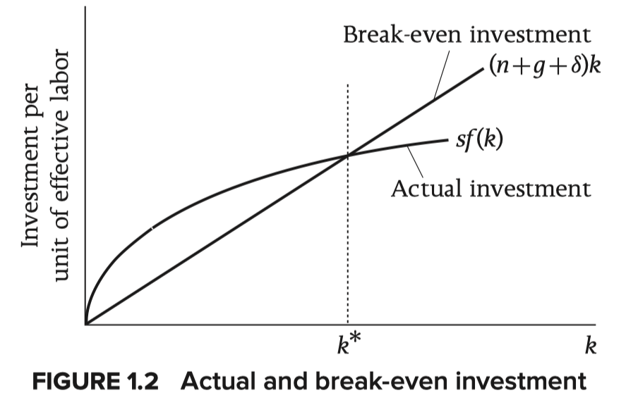
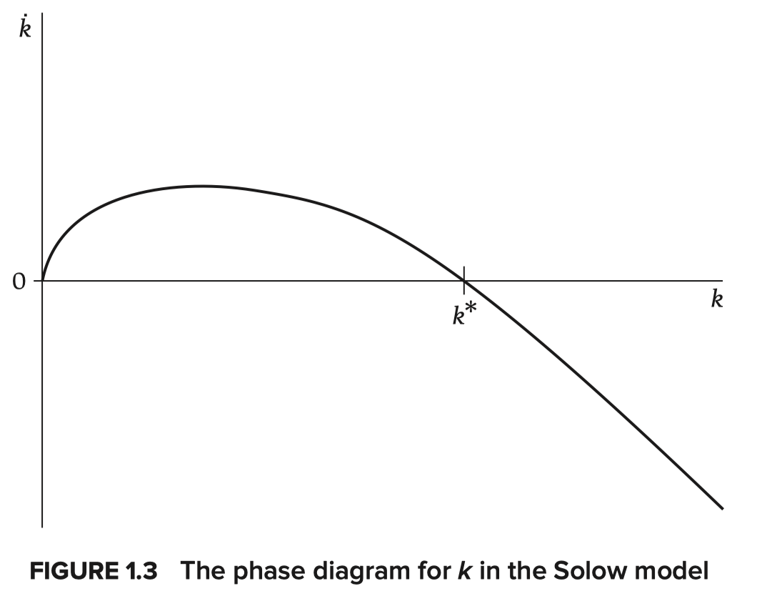
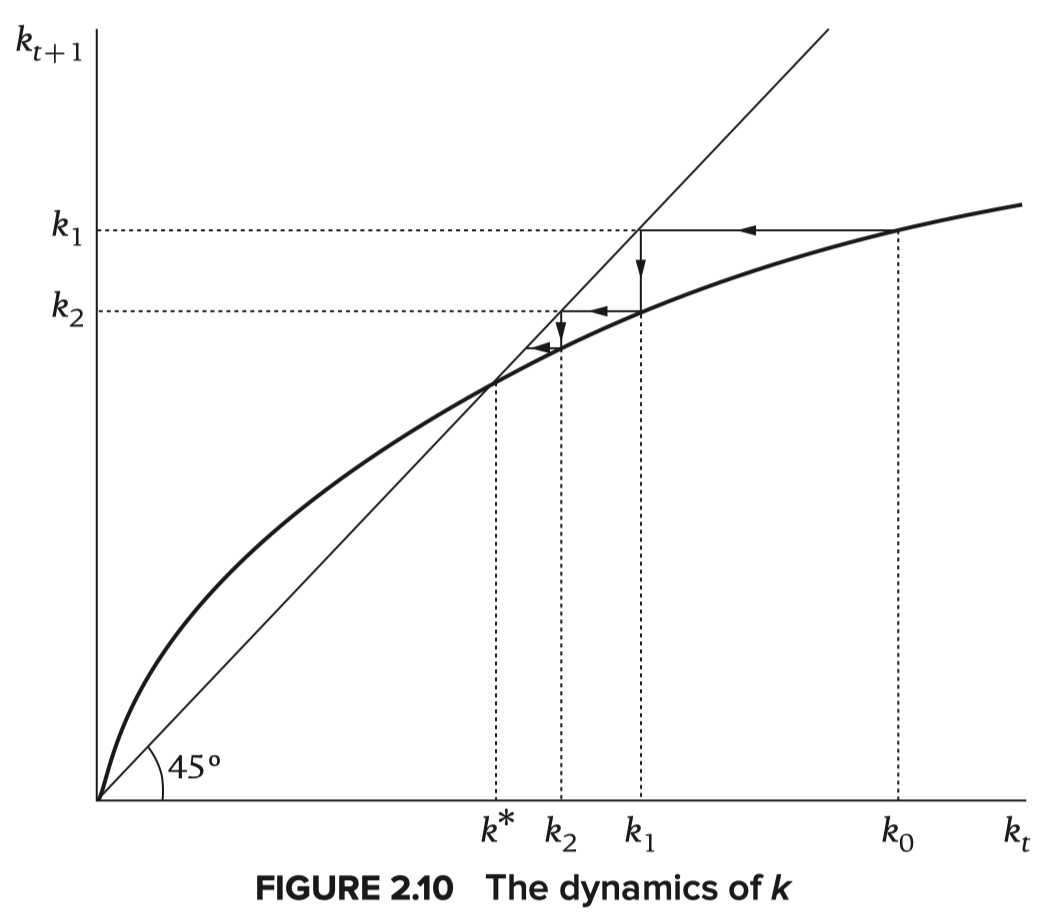
- Dynamics of : , actual investment - breakeven investment.
- To satisfy the assumptions above, there must be one and only one intersect of actual and breakeven investment, the point of convergence .
- Balanced growth path: each variable of the model is growing at a constant rate(deduced from the condition ).
- Impact of change in the saving rate: A permanent increase in the saving rate lifts the curve of actual investment(thus the value of rises, the balanced growth path changes).
- Output: produces a temporary increase in the growth rate of and . Level effect instead of Growth effect. (only technological progress have growth effect)
- Consumption: decreases immediately then rise slowly with the increase of until . Since where , increases iff (the marginal product of capital) exceeds . As increases from a low value, consumption first increases then decreases, reaching its peak when makes (the corresponding value of =the golden-rule level).
- Quantitative implications.
- , where (directly from ). Ultimately we have where denotes the elasticity of output w.r.t (namely ).
- A way to estimate: If capital earns its marginal product, the share of total income that goes to capital(on the balanced growth path) is , i.e. . The value(in most countries) is about then the elasticity of w.r.t is about .
- Speed of convergence: when , where .
- , where (directly from ). Ultimately we have where denotes the elasticity of output w.r.t (namely ).
- Conclusion: Economic growth and cross-country income differences can be explained only by the advancement/difference of the effectiveness of labor(i.e. technological progress).
- Applications:
- Growth accounting: , where denotes the elasticity of output w.r.t capital, labor, . Then , or .
- Convergence.
- Environment & economic growth:
- A baseline case: Let , where denote the resources, amount of land and when is suff large. Then .
- , therefore when exceeds its BGP value, falls, causing ‘s decrease, thus can finally converge to its BGP value.
- , that means technological advance serves as a spur and land/resource limitation as a drag.
- An illustrative calculation: Consider a compared economy where . Here , then . Actually the influence of such drag is somewhat smaller that imagination.
- A complication:
- A baseline case: Let , where denote the resources, amount of land and when is suff large. Then .
Ch2 Part A The Ramsey-Cass-Koopmans Model
- Assumptions: (differences only)
- No depreciation(only for convenience): , here denotes total consumption.
- Firms: They all have a common production function and common prices for all factors; CRS holds. Thus total output . Firms maximise profits. Since they are owned by households, any profits earned accrue to the households.
- Households: The size of each grows at rate . Each member supplies unit of labor. It rents every capital it owned to firms(with initial capital holdings of ). Consumption + saving = labor + capital income. Utility function: , where =consumption of each member, =instantaneous utility function(utility of each member at a given date), =total population(= members of the household), =the discount rate.
- , the CRRA(constant-relative-risk-aversion) utility.
- Behaviours:
- Firms: (with CRS, Euler’s theorem implies then firms have zero profits), , .
- Households:
- Budget constraint: , where =labor earning per person(=), =consumption per person(=). Since the household’s wealth at time is , the constraint can be written in the form of (no-Ponzi-game condition).
- Maximisation: , where and . , or . When lifetime utility is maximised, the budget constraint takes the equality. Set , the first-order condition for is . Take logs and take derivative w.r.t. , (Euler Equation). Then . Here satisfies and is determined by .
- Dynamics:
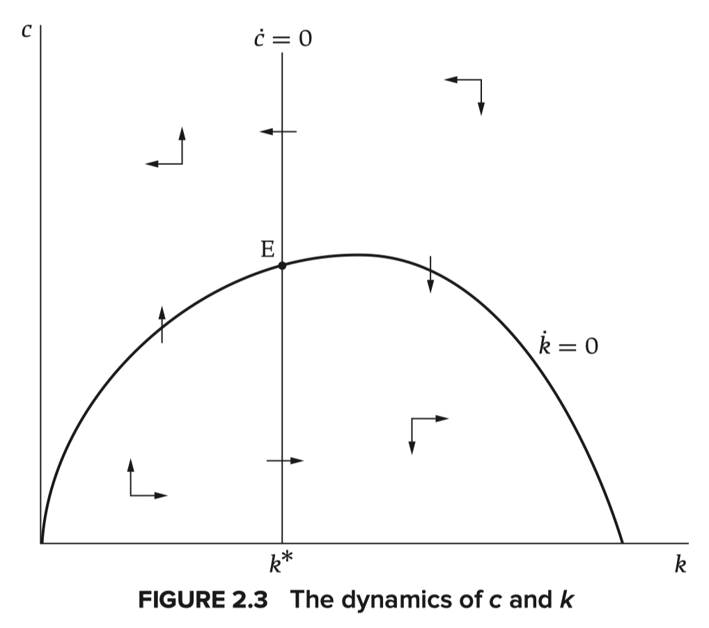
- : . Let when . Then is rising when , falling when .
- : . is rising in when , falling when .
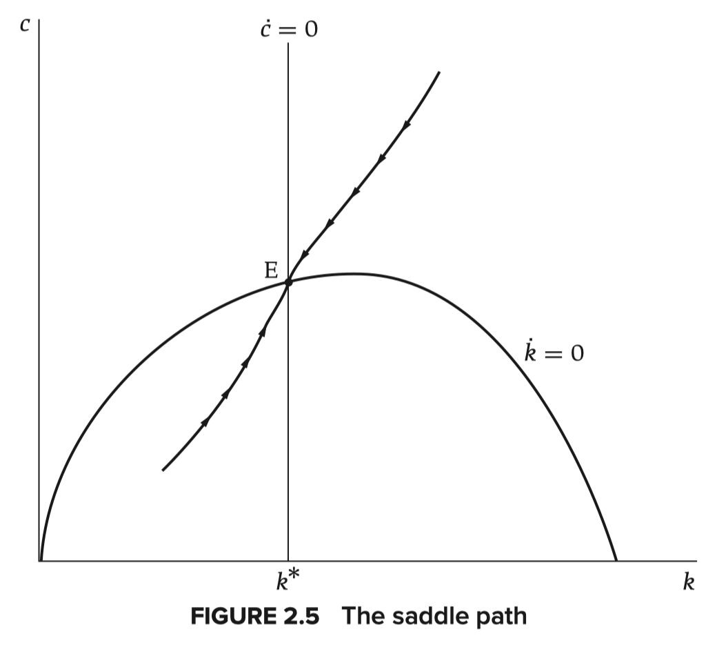
- The phase diagram(given initial values of ): Here the peak of the curve is which satisfies (when reaches its peak under the condition of equilibrium). Since and is decreasing in , . The origin, intersection of and and E are stationary point().
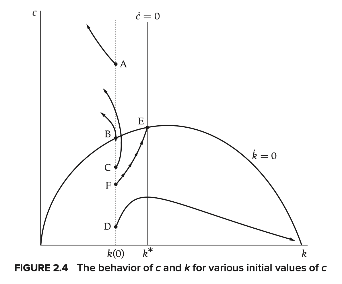
- The initial value of : When starts at a point above F, would eventually be negative; below F, indicating that the utility function has not maximised. Therefore can only be at the level of F, constituting the saddle path.
- Efficiency: For social planners who control the allocation between directly, to reach Pareto efficiency is to find an allocation path to maximise under the constraint . Households’ and firms’ behaviour yield the same result. Since planner’s choice can maximise the welfare, the competitive equilibrium maximises it as well. (the first welfare theorem with dynamics taken into account)
- The balanced growth path: Once the economy converges to point E, are constant and the result of Solow model can be applied.
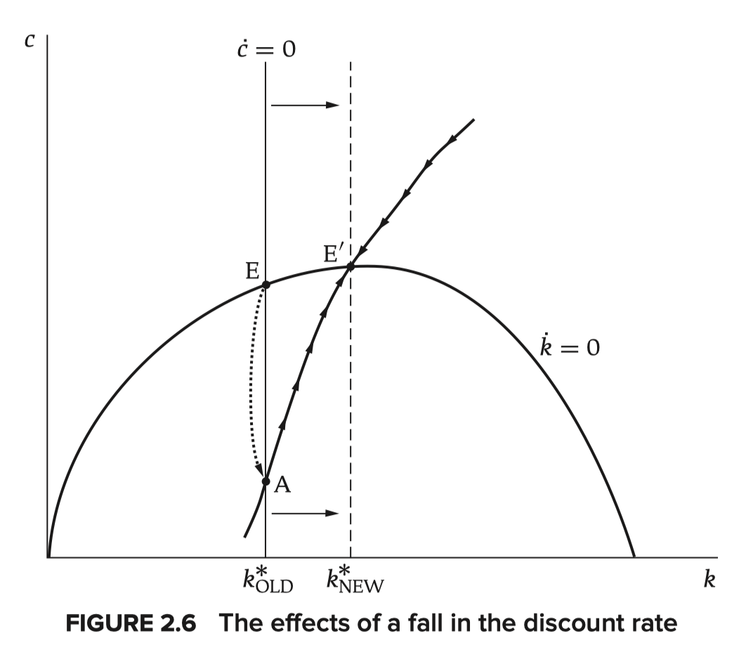
- The effects of a fall in the discount rate: Note that the stock of capital cannot change discontinuously. Let . Around the BGP we have . Substitute the dynamics of in, , or .
- When rise/fall at a same rate, remains constant i.e. the economy moves along a specific line to point E. Actually has two solutions , corresponding to line AA(converge to E) and BB(away from E, omitted).
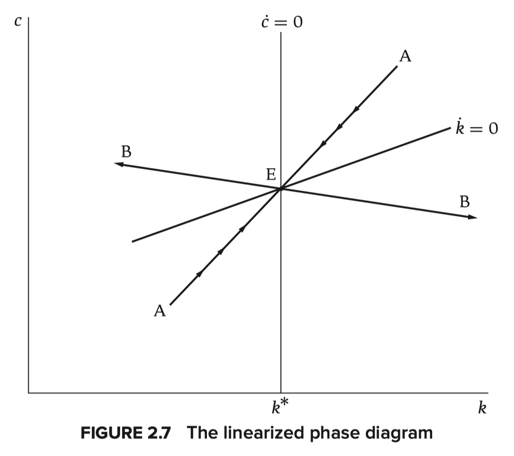
- When rise/fall at a same rate, remains constant i.e. the economy moves along a specific line to point E. Actually has two solutions , corresponding to line AA(converge to E) and BB(away from E, omitted).
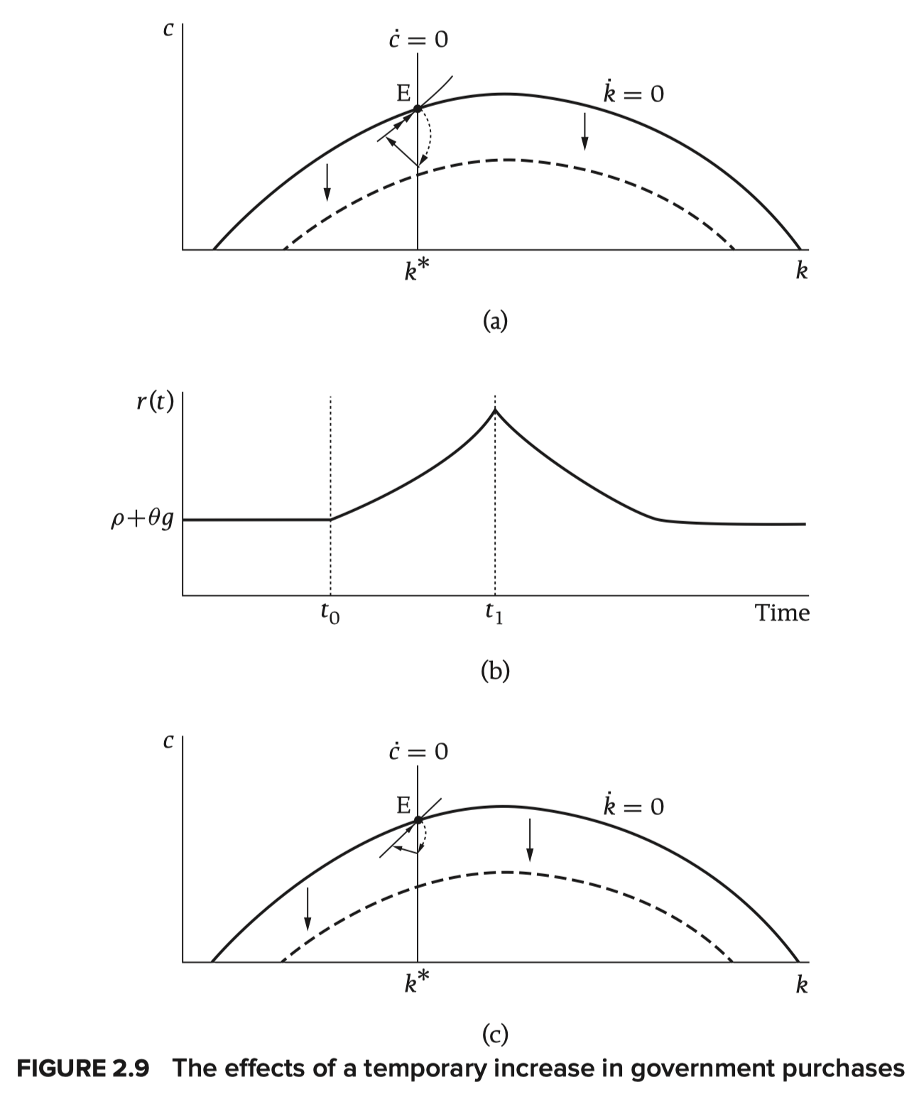
- The effects of government purchases: Gov buys output at rate (per unit of per unit time). The purchases are all devoted to public consumption; financed by taxes of amount . Then (consumption) and (tax).
- A permanent increase in : Since the implication of this increase is even in time, adjusting the time pattern of consumption won’t raise the value of . The size of the immediate fall in consumption equals . (compare the case of Solow model where such increase will crowd out investment )
- A temporary increase in : Note that cannot change discontinuously at the time that returns, otherwise the utility function wouldn’t be optimal. Households tend to pay the additional taxes from the savings(short-term, thus cut the investment, figure(c))/after reducing consumption(long-term, figure(a)).
Ch2 Part B The Diamond Model
- Assumptions: There is turnover in the population. For simplicity, time is assumed to be discrete. Each individual lives for two periods(young&old): supplies unit of labor and divides income between consumption (in the current period) and investment & consumes() the saving and interest. Then (for individuals born at time ). (Here actually means , or per )
- Utility(CRSA): .
- Household behaviour: Budget constraint . The optimisation requires , or .
- Substituting for : . Then . is increasing in iff .
- Resource constraint: Output = investment + consumption of the young + … of the old, or .
- Dynamics: .
- Simple case(logarithmic utility(), C-D production): . From Banach fixed-point theorem we know would eventually converge to .
- After the economy converges to its BGP, results of Solow model can be applied.
- A fall in results in a rise in and .
- Speed of convergence: Let , . Actually in the case below.
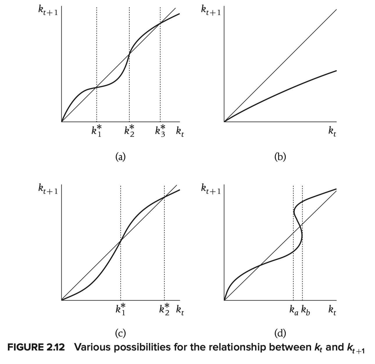
- General cases: For example in (a) are stable while is unstable.
- Simple case(logarithmic utility(), C-D production): . From Banach fixed-point theorem we know would eventually converge to .
- The possibility of dynamic inefficiency: For example with assumptions of log, C-D and , . may exceed or fall short of .
- Economy is efficient iff : The social planner chooses sequences to maximise subject to the constraint of resources. Set Lagrangian First-order conditions areHence . In steady state(), , or . When , can never be (or to say that appointing to be raises consumption in all future periods, a Pareto improvement). Otherwise there exists(guaranteed by the continuity of ) a sequence to make .